Image Details

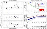
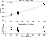
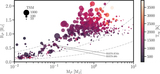
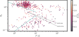
Caption: Figure 1.
Observations used to confirm the transiting planet system HATS-37. Top left: phase-folded unbinned HATSouth light curve. The top panel shows the full light curve, the middle panel shows the light curve zoomed in on the transit, and the bottom panel shows the residuals from the best-fit model zoomed in on the transit. The solid lines show the model fits to the light curves. The dark filled circles show the light curves binned in phase with a bin size of 0.002. Top right: unbinned follow-up transit light curves corrected for instrumental trends fitted simultaneously with the transit model, which is overplotted. The dates, filters, and instruments used are indicated. The residuals are shown on the right side in the same order as the original light curves. The error bars represent the photon and background shot noise, plus the readout noise. Note that these uncertainties are scaled up in the fitting procedure to achieve a reduced χ2 of unity, but the uncertainties shown in the plot have not been scaled. Bottom left: high-precision RVs phased with respect to the midtransit time. The instruments used are labeled in the plot. The top panel shows the phased measurements together with the best-fit model. The center-of-mass velocity has been subtracted. Both the observations and the model have also had a linear trend in time subtracted (Figure 5). In this case the model has not been corrected for dilution from the unresolved stellar component HATS-37B. We find that the dilution corrected orbit has a semiamplitude that is ∼20% larger than what is shown here. The second panel shows the velocity ﹩O-C﹩ residuals. The error bars include the estimated jitter. The third panel shows the bisector spans. Bottom right: color–magnitude diagram (CMD) and spectral energy distribution (SED). The top panel shows the absolute G magnitude vs. the dereddened BP − RP color compared to theoretical isochrones (black lines) and stellar evolution tracks (green lines) from the PARSEC models interpolated at the best-estimate value for the metallicity of the host. The age of each isochrone is listed in black in gigayears, while the mass of each evolution track is listed in green in solar mass units. The filled blue circles show the measured reddening- and distance-corrected values from Gaia DR2, while the blue lines indicate the 1σ and 2σ confidence regions, including the estimated systematic errors in the photometry. Here we model the system as a binary star with a planet transiting one component. The 1σ posterior distributions for the primary star HATS-37A and secondary star HATS-37B are shown as red ellipses. The gray ellipse shows the 1σ posterior distribution for the combined photometry of the system. The inset shows a zoomed-in view around the primary star and the combined photometry. The middle panel shows the SED as measured via broadband photometry through the listed filters. Here we plot the observed magnitudes with mass ﹩0.84﹩ ﹩{M}_{\odot }﹩, and a secondary star with mass ﹩0.65﹩ ﹩{M}_{\odot }﹩. The second mode consists of a primary star with mass 0.88 ﹩{M}_{\odot }﹩, and a fainter secondary star with mass 0.48 ﹩{M}_{\odot }﹩. The first mode is ∼35 times more likely based on its representation in the posterior distribution. The model makes use of the predicted absolute magnitudes in each bandpass from the PARSEC isochrones, the distance to the system (constrained largely via Gaia DR2) and extinction (constrained from the SED with a prior coming from the MWDUST 3D Galactic extinction model). The bottom panel shows the ﹩O-C﹩ residuals from the best-fit model SED.
Other Images in This Article
Copyright and Terms & Conditions
© 2020. The American Astronomical Society. All rights reserved.