Image Details
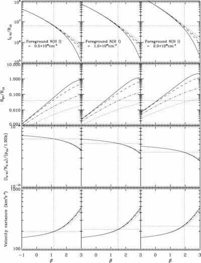
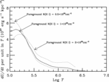
Caption: Fig. 4.
Sensitivity of various physical parameters on the values of observed quantities. The three columns of panels represent solutions of the equations assuming different values for the foreground absorption, represented by ﹩N_{\mathrm{H}\,\,{}^{{\rm{\small I}}}}﹩: left, ﹩0.5\times 10^{20}﹩ cm−2; middle, ﹩1.0\times 10^{20}﹩ cm−2; and right, ﹩2.0\times 10^{20}﹩ cm−2. In all of the plots, curves for different assumed values of ﹩T_{\mathrm{cut}\,}﹩ are drawn in different styles: solid curves, ﹩\mathrm{log}\,T_{\mathrm{cut}\,}=8.0﹩; dashed curves, ﹩\mathrm{log}\,T_{\mathrm{cut}\,}=6.9﹩; dash‐dotted curves, ﹩\mathrm{log}\,T_{\mathrm{cut}\,}=6.6﹩; and dotted curves, ﹩\mathrm{log}\,T_{\mathrm{cut}\,}=6.4﹩. Top: Dependence of β on the value of ﹩I_{\mathrm{O}\,\,{}^{{\rm{\small VI}}}}/ R_{12}﹩ in units of O VI photons arcmin2 R12 counts−1 sr−1, as defined in eq. (8). From the intersection of the observed value of this ratio (horizontal dotted line) and the curves, we obtain the best values of β in each case (vertical dotted lines dropped down to the β scales at the bottom). Second row: Dependence of ﹩T_{\mathrm{cut}\,}﹩ on ﹩R_{67}/ R_{12}﹩ as a function of β, as defined by eq. (9). We used these curves to define appropriate values of ﹩T_{\mathrm{cut}\,}﹩ in each case by locating the one that most closely intersects the horizontal dotted line representing the observation at the preferred value of β. Third row: Expected ratio ﹩( I_{\mathrm{O}\,\,{}^{{\rm{\small VI}}}}/ N_{\mathrm{O}\,\,{}^{{\rm{\small VI}}}}) / ( p_{\mathrm{th}\,}/ 1.92k) ﹩ as a function of β, as expressed in eq. (10). The intersections of the dotted lines show the outcomes for the best β‐values with the thermal pressures listed in Table 4. Bottom: Expected velocity variance as a function of β, as defined in eq. (11).
Other Images in This Article
Copyright and Terms & Conditions
© 2007. The American Astronomical Society. All rights reserved. Printed in U.S.A.