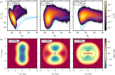
(a) Distribution of (T_⊥e/T_∥e, β_∥e) for electrons at ﹩t=0.5{\tau }_{{\rm{\exp }}}﹩ (left), ﹩t=1.0{\tau }_{{\rm{\exp }}}﹩ (middle), and ﹩t=1.5{\tau }_{{\rm{\exp }}}﹩ (right). The distribution is scaled as the amount of cells (n_c) normalized by the total amount of cells (N_c). Isocontours of the theoretical oblique EFI are plotted as blue lines with ﹩{T}_{\perp e}/{T}_{\parallel e}=1-1.29/{\beta }_{\parallel e}^{0.97}﹩ (dotted), ﹩{T}_{\perp e}/{T}_{\parallel e}=1-1.32/{\beta }_{\parallel e}^{0.61}﹩ (dashed), and ﹩{T}_{\perp e}/{T}_{\parallel e}=1-1.36/{\beta }_{\parallel e}^{0.47}﹩ (solid) associated with growth rates of γ = 0.001, 0.1 and 0.2Ω_e, respectively (S. P. Gary & K. Nishimura 2003), with Ω_e = eB/(m_ec) and e is the electron charge. The green dashed line corresponds to the double-adiabatic expansion prediction (﹩{T}_{\perp e}/{T}_{\parallel e}={\beta }_{\parallel e}^{-1}﹩). (b) Logarithmic ratio between the electron VDFs (f) and a reference Maxwellian VDF (f_M) in (v_⊥e, v_∥e)-space at ﹩t=0.5{\tau }_{{\rm{\exp }}}﹩ (left), ﹩t=1.0{\tau }_{{\rm{\exp }}}﹩ (middle), and ﹩t=1.5{\tau }_{{\rm{\exp }}}﹩ (right).