Image Details
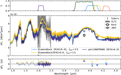
Caption: Figure 2.
Comparing the spectrum of 29 Cyg b to atmospheric models. Top: the transmission functions of the photometry considered in the fit. Middle: RCE models from Sonora Diamondback are shown in blue and yellow, and a parametric model generated with petitRADTRANS is shown in purple. Observations from Subaru, the VLTI, Keck, and JWST are plotted in black and gray, and the models integrated across the filter transmission functions are shown as the smaller colored scatter points. The maximum a posteriori spectrum (a linear interpolation across the published grid of spectra, with [M/H] = 0.43 and fsed = 2.5) is shown in blue, and a similar model with a solar metallicity ([M/H] = 0.0) and stronger cloud sedimentation (fsed = 1.5) is shown in yellow. The median model has a reduced χ2 = 1.0. The models with enhanced metallicity in the Diamondback grid provide a better fit to the absorption feature from CO2 at 4.3 μm, while the metallicity-dependent JHK-band spectral slope could be reproduced by changing the model’s cloud parameters (in this case, the sedimentation efficiency fsed). The more flexible P-T structure and cloud parameterization in the best-fitting pRT model are able to reproduce the K-band observations, the JHK-band spectral slope, and the 4–5 μm photometry at once, while preserving the surface gravity and radius predicted by the dynamical mass and evolutionary models. The median pRT model has a reduced χ2 = 1.0. Bottom: residuals (in units of standard deviation) between the models and the observations as a function of wavelength.
Other Images in This Article
Copyright and Terms & Conditions
© 2026. The Author(s). Published by the American Astronomical Society.