Image Details
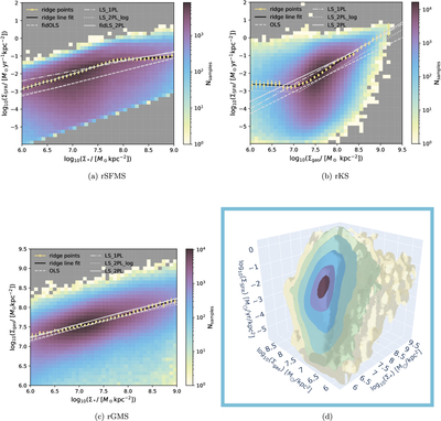
Caption: Figure 1.
(a–c) The rSFMS, rKS, and rGMS scaling relations, respectively, from our fiducial maps, which demonstrate the ridge line and ordinary least-squares fitting techniques. The 2D histogram shows the number of spaxels (i.e., samples) in bins of values on the x- and y-axes. Yellow points indicate the “ridge” or conditional mode of the data, and the black line shows the double linear fit to those ridges. Uncertainties on the ridge points are estimated as the bandwidth of the KDE obtained with Scott’s rule (D. W. Scott 1979). The gray lines show least-squares fits to a single power law (dashed and dotted–dashed lines) and to a double power law (dotted and solid lines) using the full data set in linear space (dotted–dashed and solid) and in ﹩{\mathrm{log}}_{10}﹩ space (dashed and dotted). (d) A 3D visualization of the relationship between Σ*, Σgas, and ΣSFR. Isodensity contours are drawn at the 50th, 70th, 85th, 95th, and 99.9th percentiles. In the online article, this panel is available as an interactive figure, where the 3D visualization can be rotated.
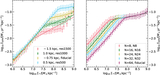
An interactive version of this figure is available in the online article.
An interactive version of this figure is available.
An interactive version of this figure is available in the online journal.
Other Images in This Article
Copyright and Terms & Conditions
© 2025. The Author(s). Published by the American Astronomical Society.