Image Details
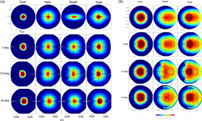
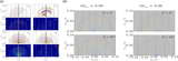
Caption: Figure 3.
(a) Interaction of solar wind electron distributions at 1 au with single whistler wave. Top panels show the initial distributions. The next panels show the distributions after interacting with an almost parallel (in the direction of strahl), antiparallel (opposed to the strahl), and very oblique wave for 60 wave periods. The white x's indicate the location where the n = −1, 0, and 1 resonances intersect ﹩{v}_{\perp }=0﹩. The black circles plot constant energy in the wave frame. (b) Interaction of solar wind electron distributions at 0.3 au with single whistler wave. The top panel shows the initial distributions for core, strahl, and total distributions at t = 0. The next panels show the distributions after interacting with an almost parallel (in the direction of strahl), antiparallel (opposed to the strahl), and very oblique wave for 60 wave periods. The white x's indicate the location where the n = −1, 0, and 1 resonances intersect ﹩{v}_{\perp }=0﹩. The black circles plot constant energy in the wave frame.
Other Images in This Article
Copyright and Terms & Conditions
© 2021. The Author(s). Published by the American Astronomical Society.