

Image Details
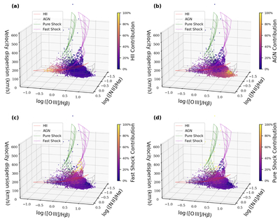
Caption: Figure 1.
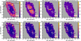
Distribution of MUSE IFU data for IC 5063 on the theoretical 3D diagram, with spaxels color coded by the fractional contributions of H II regions (top left), AGN (top right), fast shocks (bottom left), and pure shocks (bottom right). The H II models with ﹩\mathrm{log}(P/k)=6.0﹩, AGN models with ﹩\mathrm{log}(P/k)=7.4﹩ and ﹩\mathrm{log}{E}_{\,{\rm{peak}}\,}\,\,{\rm{keV}}{\,}^{-1}=-1.0﹩, fast-shock, and pure-shock model grids with ﹩\mathrm{log}(P/k)=10.2﹩ and ηM = 0.0001 are overplotted in red, gray, magenta, and green, respectively, showing lines of constant metallicity (﹩12+\mathrm{log}({\rm{O}}/{\rm{H}})=8.12,8.42,8.82﹩ for the H II model; ﹩12+\mathrm{log}({\rm{O}}/{\rm{H}})=8.43,8.70,8.80,9.02,9.26﹩ for the AGN and shock models), constant ionization parameter (﹩\mathrm{log}({\rm{U}})=-3.75﹩ to −2.25 in steps of 0.25 dex for the H II model and ﹩\mathrm{log}({\rm{U}})=-3.8﹩ to −2.2 in steps of 0.4 dex for the AGN model), and constant shock velocity (Vs = 158, 179, 202, 228, 257, 290, 328, 370, 418, 472, 533, 601, 678, 766 km s−1) for the shock models. The x- and y-axis ranges are tailored to encompass the full range of IFU data and theoretical models, as shown clearly in the interactive version of this figure, available in the online journal. The interactive version of this figure allows the reader to zoom and rotate any of the four panels. Hovering the mouse over a point displays the object name and its x, y, and z coordinates. In addition, the standard Plotly toolbar commands are available, including the option to reset the view to the default orientation.
An interactive version of this figure is available in the online article.
An interactive version of this figure is available.
An interactive version of this figure is available in the online journal.
Other Images in This Article
Show More
Copyright and Terms & Conditions
© 2026. The Author(s). Published by the American Astronomical Society.

