Image Details
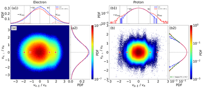
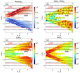
Caption: Figure 6.
Particle velocity distributions corresponding to the spatial region (x = 0–2di, y = 0–2di). (a) Electron 2D velocity distribution in the v∥ − v⊥ space. Red crosses mark fast magnetosonic speed vf and resonant speed ﹩{v}_{{\rm{res}}}﹩. (a1) Electron parallel velocity distribution, with dashed lines indicating vf and ﹩{v}_{{\rm{res}}}﹩. The light red lines indicate the difference between the two histograms. (a2) Electron perpendicular velocity distribution. The blue histogram shows the initial distribution at t = 0, and the red histogram corresponds to t = 1.55τA − 1.6τA. (b) Proton 2D velocity distribution in the v∥ − v⊥ space. Red crosses mark vf and ﹩{v}_{{\rm{res}}}﹩. (b1) Proton parallel velocity distribution, with dashed lines indicating vf and ﹩{v}_{{\rm{res}}}﹩. (b2) Proton perpendicular velocity distribution. The blue histogram shows the initial distribution at t = 0, and the red histogram corresponds to t = 1.55τA − 1.6τA. The green dashed lines represent a kappa distribution fit with κ = 4.2.
Other Images in This Article
Copyright and Terms & Conditions
© 2026. The Author(s). Published by the American Astronomical Society.