Image Details
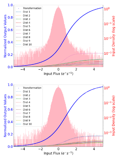
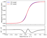
Caption: Figure 6.
Example transformations from the adaptive normalization layer for the NT model (top) and the ST model (bottom). The histogram of the input data (median-subtracted flux of a randomly selected sample) is shown in red, with density corresponding to the y-axis on the right side. Each of the 10 weighted logistic CDFs are shown as dashed lines, with the weighted sum shown in blue, all corresponding to the y-axis on the left side. The parameters of the logistic CDFs are shown in Table 2.
Other Images in This Article
Show More
Copyright and Terms & Conditions
© 2026. The Author(s). Published by the American Astronomical Society.
Copyright ©
2026 Astronomy Image Explorer. All Rights Reserved.