Image Details
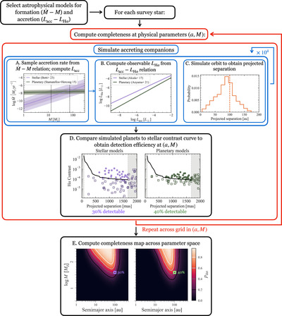
Caption: Figure 1.
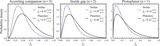
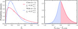
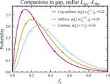
Workflow for estimating direct-imaging survey completeness to accreting companions. First, select models for ﹩\dot{M}-M﹩ and LHα − Lacc, corresponding to assumptions about formation and accretion. Estimate the completeness for each survey star with the following Monte Carlo procedure. At each set of physical parameters (a, M), simulate 104 accreting companions. (A) Sample mass accretion rates ﹩\dot{M}﹩ using an assumed model for the ﹩\dot{M}-M﹩ scaling. We take the empirical fit of S. K. Betti et al. (2023) as a more “stellar” scenario (purple) and the result of D. Stamatellos & G. J. Herczeg (2015) as a more “planetary” model (green; for both, see Section 2.2). The colored bands are the 1σ and 2σ uncertainties. We convert each ﹩M\dot{M}﹩ to Lacc (Section 2.3). (B) Compute the observable LHα based on a model for the accretion scaling. This is either (see Section 2.4) an empirical, stellar magnetospheric scaling (purple; J. M. Alcalá et al. 2017) or a theoretical planetary relation (green; Y. Aoyama et al. 2021). (C) Obtain the projected separation distribution by sampling the companion orbital parameters (Section 2.5); the histogram is an example for an object at a = 100 au with eccentricities following E. L. Nielsen et al. (2019). (D) Next, compare the simulated companions to the star’s contrast curve(s) to estimate the detectable fraction. The panel shows two examples of 100 brown dwarfs with (a, M) = (100 au, 40 MJ) around TW Hya; the left image shows companions simulated using both “stellar” models, while the right image uses both “planetary” models. The light circles are recovered synthetic companions, while the dark squares are undetected. (E) Repeat across a grid in (a. M) for each combination of models, to obtain the entire completeness map. Take the average across the survey stars. Repeat for each combination of astrophysical models of interest.
Other Images in This Article
Copyright and Terms & Conditions
© 2025. The Author(s). Published by the American Astronomical Society.