Image Details
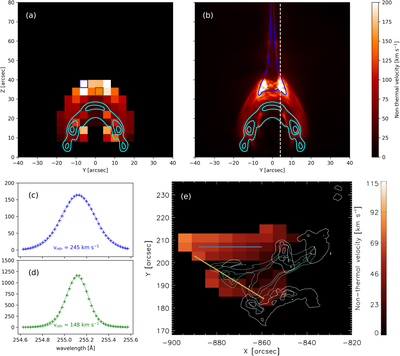
Caption: Figure 2.
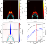
(a) Nonthermal velocity distribution obtained from Gaussian fitting of synthesized EIS/255 spectra, where the fitting method refers to Stores et al. (2021). (b) Nonthermal velocity distribution obtained from plasma density/velocity distribution. Cyan contours in (b) give the locations of the bright loop in Figure 1(b), where the contour lines show the intensity levels 25%, 50%, and 80% of peak 131 Å flux. The regions inside the blue contour have an average magnetic-field strength lower than 25 G. The green line gives the approximate location of termination shock (also see Figure 5(c)), but note that the shock locations are different at different X-slices due to interactions between reconnection outflows and magnetic arcades. Panel (c) gives the EIS/255 spectrum inside the blue box in (a), and (d) gives the spectrum inside the green box in (a) (marked with “+”). Solid lines show Gaussian fitting results of the spectra. Panel (e) shows a nonthermal velocity map from the EIS/255 spectra of an observed flare, where the cyan contours give the location of hot/dense flare loop, and white contours give the location of footpoints at the solar surface, as taken from Stores et al. (2021). The spatial resolution of the synthesized EIS/255 data is reduced before fitting, as in Stores et al. (2021). Panel (a) has a pixel size of 4″ × 4″, which is close to that in panel (e) (6″ × 4″). Panel (b) has a smaller pixel size of 0.″138 × 0.″138. An animation of this figure is available, showing the evolution of spatial average electron number density in x-direction (panel (a)) and nonthermal velocity distribution obtained from plasma density/velocity distribution (panel (b)). The contours in the panels show the intensity levels 10%, 25%, 50%, and 80% of peak 131 Å flux. The animation covers 2.37 minutes of physical time starting at t = 7.51 minutes (real-time duration 3 s).
(An animation of this figure is available.)
The video/animation of this figure is available in the online journal.
Other Images in This Article
Copyright and Terms & Conditions
© 2023. The Author(s). Published by the American Astronomical Society.