Image Details
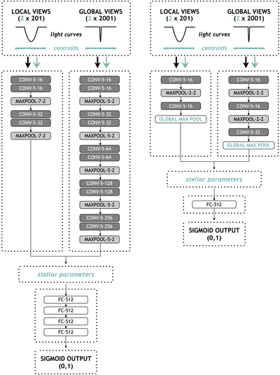
Caption: Figure 2.
Convolutional neural network architectures used in this Letter. Left: Exonet, where the additions over the baseline Astronet model are shown in blue (Section 3.2). The flattened outputs of the disjoint one-dimensional convolutional columns are concatenated with the stellar parameters, then fed into the fully connected layers ending in a sigmoid function. Following Shallue & Vanderburg (2018), the convolutional layers are denoted as CONV–﹩\langle \mathrm{kernel}\,\mathrm{size}\rangle ﹩–﹩\langle \mathrm{number}\,\mathrm{of}\,\mathrm{feature}\,\mathrm{maps}\rangle ﹩, the max pooling layers are denoted as MAXPOOL–﹩\langle \mathrm{window}\,\mathrm{length}\rangle ﹩–﹩\langle \mathrm{stride}\,\mathrm{length}\rangle ﹩, and the fully connected layers are denoted as FC–﹩\langle \mathrm{number}\,\mathrm{of}\,\mathrm{units}\rangle ﹩. Right: the significantly reduced Exonet-XS model version described in Section 3.3.
Other Images in This Article
Copyright and Terms & Conditions
© 2018. The American Astronomical Society. All rights reserved.